Branch Switch
Branch switch in FEAP is possible if one use arclength continuation methods. Here is a simple example. Consider a built-in column with an axial load.
feap ** Buckling Path Following with Arclength **
0 0 0 3 3 8

para
 e = 1.0
 d = 0.5
 h = 20
 pi = 4.*atan(1.)
 i  = 16.*d*d*d*d/12
 pe = pi*pi*e*i/h/h/4       ! Euler load
 p  = 0.1*pe/4/d/d          ! Reach euler load a prop value of 1


mate
 solid
  elastic moon e 0.4 0.05
  finite
  mixed

block
 cart 4 4 20*2
 1 -d -d 0
 2  d -d 0
 3  d  d 0
 4 -d  d 0
 5 -d -d h
 6  d -d h
 7  d  d h
 8 -d  d h

eboun         ! Fixed base
 3 0 1 1 1

csur          ! Pressure load (dead)
 surface
 1 -d -d h -p
 2  d -d h -p
 3  d  d h -p
 4 -d  d h -p

end
As set up the buckling load occurs according to Bernoulli-Euler theory when the load factor reaches 10. If one simply applies the load in FEAP to this level and beyond the computed solution will just be a compression of the column, though above a load of 10, FEAP will report
*D4TRIU WARNING* Sign of diagonal changed when reducing 2 equations.
due to the two lowest buckling modes. As the load increases more modes can present themselves and more equations will be reported to have sign changes during the solution process. Though FEAP detects the multiple solutions it will typically only find the unstable vertical solution. In order to bump onto the bifurcation branches one can use ARCLength and the ADD feature.
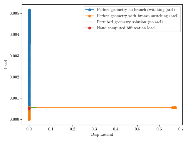
The basic process is to run the load up to where the bifurcation point is thought to be. Then after solving on to the suspected unstable branch, one computes the lowest eigenvector. This is then added to the current solution and the problem is re-solved (without increasing the load). If the eigenvector points in the direction of a bifurcation solution, one will likely converge upon it. Once on the bifurcation solution, if it is stable, increases in load should stay on the new path (without the need for guidance from further eigenvectors).
With the example give above, one can perform this process with the following algorithm
batch
 opti          ! Optimize the equation ordering for the profile solver
 tplo          ! Set up time-history plots
end
arcl 1 1       ! Save the arclength parameter to file
disp 1025 1    ! Save the corner x displacement
disp 1025 2    ! Save the corner y displacement
show


batch
 dt,,1
 arcl,,2         ! Initiate ARCLength
 loop,,10        ! 10 steps to get near buckling load
  time
  loop,,30
   tang,,1
  next
  plot,pview     ! Save the state for paraview plotting
 next
!
 loop,,2         ! 1 Steps using the eigen method to probe for a bifurcation path
 time
 loop,,30
  tang,,1
 next
 iden
 subs            ! Get eigenvalues and vectors
 arcl,add,1,.1   ! Pertub onto first eigenvector hope it is the stable branch
 loop,,30        ! Re-converge
  tang,,1
 next
 plot,pview      ! Save the state for paraview plotting
 next
!
 loop,,5         ! Take 5 more steps on hopefully the stable buckling branch
  time
  loop,,30
   tang,,1
  next
  plot,pview     ! Save the state for paraview plotting
 next
end

inte

stop
Here is a comparison of the solution techniques just mentioned in terms of axial load versus transverse motion.
